Month 1 Report: Initial AutoMATES architecture, algorithms, and approaches
02 Dec 20181. Architecture Overview
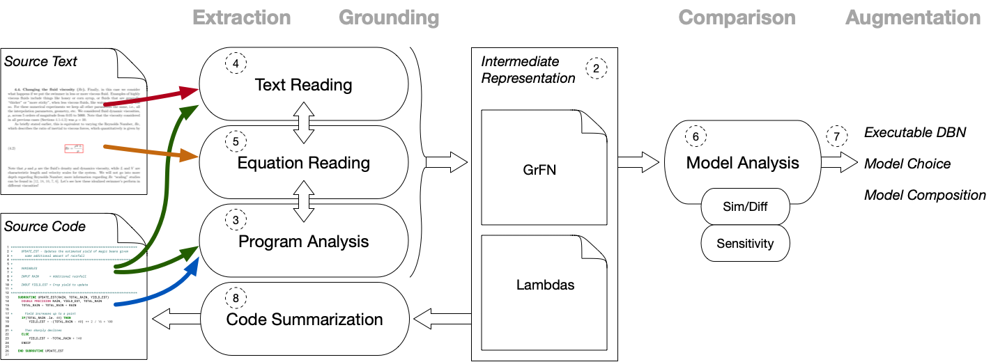
The architecture of the AutoMATES system is summarized in the figure above.
On the far left are the two information sources that serve as inputs to the system: documents containing text and equations that describe scientific models, and source code containing program instructions and natural language comments that implement said models.
Along the top of the figure are four headings (in grey) that describe the general type of processing being carried out by AutoMATES in the columns below the heading:
- Extraction of information from the input data sources (text and source code).
- Grounding the extracted information by linking between information types (text, equations and source code) and connecting identified terms to scientific domain ontologies.
- Comparison of models by analyzing structural and functional (via sensitivity analysis) similarities and differences.
- Augmentation of models through selection of model components appropriate for a task, composing model components, and model execution; AutoMATES produces executable model components (as dynamic Bayesian networks) and provides results of Comparison, but in the ASKE program selection and composition will be done manually by humans.
Extraction and Grounding are performed by three interacting pipelines: Program Analysis, Text Reading and Equation Reading.
- The Program Analysis pipeline extracts program source code and associated comments and performs an analysis that identifies variables and the functional relationships between them, as determined by program control flow and expressions. This results in a Function Network representation of the variable relationships paired with modular functions that compute the variable states (Lambdas). Within the ASKE program, the AutoMATES Program Analysis pipeline will focus on extraction and analysis of Fortran source code. Additional language processing pipelines can be modularly added in the future, with each language pipeline providing language-agnostic output of the intermediate representation.
- The Text Reading pipeline processes text from papers and other documents (input as PDFs) describing scientific models as well as input comments associated with source code. This pipeline extracts contextual information about models, including identifying mentions of physical variables and grounding them to domain ontologies, and specifics about variable ranges, units, confidence scores, etc. Variable mentions identified in comments can be linked to mentions in the documents. Machine reading also extracts the context of equations, grounding mentions of variables in equations.
- The Equation Reading pipeline extracts equations from PDFs, first identifying the LaTeX source code that could produce the equation image, and then mapping the LaTeX representation to a symbolic math representation. Equation Reading interacts with the Program Analysis pipeline by passing along the symbolic mathematical representation to perform the same analysis that extracts the source code Function Network and Lambdas, and interacts with the Text Reading pipeline to ground equation variables to their context in the source text discourse.
The result of the coordinated Extraction and Grounding pipelines is a unified, programming language-agnostic intermediate representation that explicitly links the extracted information in the scientific discourse context and variables grounded in domain ontologies with the Function Network and Lambdas extracted in program analysis and equation extraction. The Grounded Function Network (GrFN) intermediate representation captures all of this linked information in a form that permits further model analysis.
Model Comparison and eventual Augmentation is then enabled by the Model Analysis pipeline. The goal of this pipeline is to take GrFN and Lambdas representations of extracted source models and their descriptions, and enable efficient model comparison: identifying what portions of two or more models share same or similar computations about similar variables, and which components are different. The GrFN representation is first analyzed according to the structural properties of the Function Network: shared grounded variables between two models are identified and the function network topology is analyzed to identify which computations involved in setting variable states are similar and which are different. Then, the Lambdas are incorporated to analyze the functional relationships between variables in similar networks, through sensitivity analysis. Because sensitivity analysis can be computationally expensive, automatic code differentiation will be used to efficiently compute the derivatives (rates of change) of variables with respect to each other, and Bayesian optimization techniques will be used to estimate sensitivity functions with as few samples as possible. The final product of this analysis (1) includes modular executable representations of grounded models (as dynamic Bayesian networks), (2) provides results of model comparison to enable model choice in tasks, and (3) based on grounded model similarity and differences, enables model composition.
Finally, the combined, grounded information in the GrFN representation that is linked to the original source code is the basis for generating natural language summaries of portions of the original source code. This can help improve human readability and debugging of the source code.
The following sections in the remainder of this report describe the components of the architecture in detail. The numbers in the architecture summary figure correspond to the number of the section that describes the component.
2. Intermediate Representation
The Intermediate Representation is the focal point of the AutoMATES representation: it is the programming language-agnostic target of Extraction and Grounding processes, capturing the model context by linking all of the information extracted from the input information sources, and serves as the basis for contextualized model analysis and Augmentation. This information is combined in the unified The Grounded Function Network (GrFN) representation. The modular representation of variable-setting functions in the Lambdas representation is described in the next section on Program Analysis; Lambda function modules are referred to in the GrFN specification of a model.
We use a JSON format for the GrFN specification for simple serialization, deserialization, and compatibility with web APIs. The current state of the GrFN specification is described here: GrFN specification
3. Program Analysis
Analyzing Fortran Source Programs: for2py
for2py is a front-end translator that maps Fortran source programs to
a language-independent program analysis intermediate representation
(PAIR) that is then used to generate files used as input to subsequent
analysis. The PAIR currently consists of Python data structures
representing the abstract syntax of the input code, together with
comments extracted from the source files, that are saved as pickled
Python files. The output generated by for2py includes GrFN JSON files
and representations of modular computations from the source code being
analyzed (Lambdas).
The for2py pipeline is implemented within the public
Delphi project, under the
delphi/program_analysis/
sudirectory.
Program Analysis Intermediate Representation
While for2py targets programs written in Fortran, the PAIR to which it
maps the source code aims to avoid language-specific assumptions. An
important design principle for our PAIR is to retain, as much as possible,
the high-level computational structure of the input code while
abstracting away language-specific details. Retaining the high-level
computational structure of input programs makes it easier to perform
high-level qualitative analyses and to connect information about
constructs in the input code, e.g., variables or subprograms, with the
results of analyses of text documents and equations. The
language-independent nature of the PAIR makes it possible (in principle)
to analyze models that may have been implemented using multiple source
languages, and also to reason about and compare models written in
different programming languages.
Processing Pipeline
The translation process in for2py is organized as the following
pipeline:
-
Input processing. [Language-dependent; currently Fortran-specific.] The source code is read in and analyzed to produce an program analysis intermediate representation (PAIR). This consists of the following steps:
-
Preprocessing and comment extraction. Preprocessing involves cleaning up or transforming source language constructs to make subsequent parsing easier and more robust. Comment extraction aims to get around the fact that most language parsers are implemented as compiler front-ends and therefore discard comments.
-
Parsing. For2py uses the Open Fortran Parser (OFP) to parse the Fortran source code into an abstract syntax tree (AST) representation that is then written out as an XML file.
-
Integration and translation to PAIR. The AST is read in from the XML files created by OFP. Various tree transformations are applied: both to abstract away a number of language-specific details (e.g., the way in which function return values are indicated in Fortran), and also to address some bugs in OFP. The transformed ASTs are integrated with comments extracted in the first step listed above. In addition to this, the entry-points for the Fortran source file are determined and the resulting PAIR is then serialized to a Python pickle file. (Note: the API permits bypassing this step if caching of intermediate results is not needed - for example while analyzing smaller programs.)
-
-
Output generation. [Language-independent.] The files containing the pickled Python PAIR objects are read in and processed to generate the following output files:
- Modular functional encodings of how program variables are computed as a function of other variables (Lambdas)
- GrFN JSON files
- A Python script equivalent in functionality to the Fortran file being translated (and used to verify functional behavior equivalency with original source code)
The separation of the input processing and output generation into two distinct steps is motivated by the following design considerations:
- Performance and scalability. Modules that are referenced by multiple program components do not have to be reanalyzed separately for each referencing component. Independent source-language modules can, in principle, be analyzed concurrently.
- Support for source-language heterogeneity. This design makes it possible, in principle, to support programs with different components written in different languages. It also allows us to reason about models implemented in different source languages.
- Independence of back-end tasks. Different back-end analysis tasks, e.g., sensitivity analysis and comment analysis, can be carried out independently (and, if necessary, concurrently) on the PAIR.
Scripts
for2py currently uses the following scripts:
- Input processing.
for2py_pp.py: pre-processes input Fortran files.get_comments.py: extracts comments from Fortran files.fortran_syntax.py: handles a number of Fortran language constructs.fortran_format.py: processes Fortran I/O formatting.translate.py: processes and transforms the XML files generated by OFP, integrates comments obtained fromget_comments.py, and writes out the resulting IR as a pickled Python object.
- Output generation.
pyTranslate.py: translates the pickled Python object into a fully working Python script which is equivalent in function to the original Fortran file.genPGM.py: Reads in the converted Python script to generate the GrFN JSON file.genCode.py: Works in conjunction withgenPGM.pyto create thelambdas.pyfiles for subsequent processing.
Off-the-shelf components
for2py currently uses the following off-the-shelf components:
- Open Fortran Parser. This is an open-source Fortran parser that translates Fortran source programs to ASTs written out as XML files. This component can be replaced by other software of similar functionality.
Components we are building
Components we are building consist of the following:
-
Comment extraction. We currently extract subprogram-level comments at the heads (i.e., immediately before the beginning of the subprogram code), necks (immediately after the subprogram definition but before its body), and feet (immediately after the end of the subprogram code) of subprograms.
-
Fortran I/O translation. This is important for validation of the translation process, since it allows us to map the input Fortran code to Python code whose execution behavior can be compared with that of the original Fortran program. We currently handle the I/O constructs in the
SimpleModularcrop model. -
Fortran language processing. We currently handle single-file programs that do not use Fortran’s MODULE construct. Control flow constructs such as subprograms (subroutines and functions), conditionals, loops, and case statements are all handled.
Algorithms
Algorithms currently being used or developed in for2py include the
following:
- Regular expression construction and matching.: Regular-expression-based pattern matching is used in a number of places in lexical analysis of Fortran code, including comment processing and I/O format processing.
- Tree traversals and transformations.: Pre-order and post-order tree traversals are used for analyzing and transforming program ASTs.
4. Machine Reading and Grounding
In addition to extracting information from source code, the AutoMATES team will be automatically extracting complementary scientific information from academic papers, including the description of model-relevant equations and the variables that comprise them, along with the information required for the sensitivity analysis of the models of interest in this project (such as variable domain types, ranges, and default values, etc.). Once extracted, this information will be grounded, or linked, to the model components extracted from the original source code.
Supporting code for this pipeline will be implemented in the AutoMATES repostory.
Automatic reading of scientific discourse expressed in natural language
The scientific papers that describe the models of interest will be read to extract two different types of information: (1) contextual information relevant to the models of interest, and (2) specific descriptions of equations and variables, as well as any discussion of the relations they have with each other.
Extracting context
There is a wide range of contextual information expressed in scientific descriptions of models, including ranges and units for variables, confidence scores such as p-values, and overall context required for analysis of the executable models (variable domain types, default values, etc.). In order to extract this information, the papers, which are typically found in PDF form, will be converted to text. The team will evaluate several off-the-shelf tools for this conversion and select the one that performs the best for the intended purpose. Potential tools include (but are not necessarily limited to) GROBID, Science Parse, and Science Parse version 2.
As the PDF-to-text conversion process is always noisy, the text will then be filtered to remove excessively noisy text (e.g., poorly converted tables) using common sense heuristics (e.g., sentence length and occurrence of certain special characters). Finally, the text will be syntactically parsed and processed with grobid quantities, which identifies and normalizes text mentions of measurements.
After preprocessing, the contextual information will be extracted through the use of Odin rule grammars, which can be constructed and refined quickly. Odin grammars have proven to be reliable, robust, and efficient for diverse reading at scale in both the Big Mechanism program (with the Reach system) and the World Modeler’s program (with the Eidos system). The flexibility of Odin’s extraction engine allows it to easily ingest the normalized measurements mentioned above along with the surface form and the dependency syntax, such that all representations can be used in the rule grammars during extraction.
Extracting equation and variable descriptions
In addition to contextual information, the team will also focus on extracting the descriptions of model-relevant equations and their variables found in the scientific literature, which typically occur in the immediate vicinity of the presentation of the equations themselves. However, during the conversion from PDF to text, information about the original location of a given span of text is lost. For this reason, in order to extract these descriptions, the team will first implement a component that identifies the regions of interest in the academic documents.
Specifically, using the axis-aligned bounding box found for a given equation, the team will expand it to get the text surrounding the equation. Additionally, the PDF can be converted to text in layout-preserving mode (using Poppler’s pdf2text), which will allow the team to locate the equation identifier and therefore the text around it, as well as extract the entities and relations required for the grounding the models built by other components of our system.
Once the region surrounding the equation is identified, Odin rules will likewise be used on the text within that region to extract descriptions of the equation and the variables it contains, as well as any descriptions relations between variables.
Grounding
After extraction, it will be necessary to ground the variables and equations. There are two distinct types (or directions) of grounding that will be necessary. The first is to associate a description to a variable, and the other is to associate two variables (one extracted from source code and another from text) with each other based on their descriptions and other information such as model structure (e.g., if they are both in a denominator, etc.).
The first type of grounding will link the variables and equations found in the scientific papers with their descriptions. This is seen in the following paper excerpt that shows an example of an equation and its description:
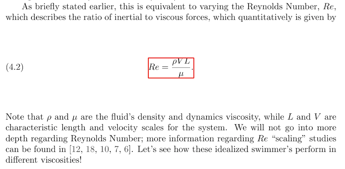
Here, each of the variables in the equation (e.g., L and V) will
be linked to their extracted descriptions (characteristic length
and velocity scales). Additionally, the entire equation will be
linked to its description (Reynolds Number). Any other instances of
these variables or equations in the text document will also be linked,
under the assumption of one sense per
discourse. Likewise, variables
occurring in the source code will be linked with any comments that
describe them.
The variables and equations from each of these sources (code and text)
will then be matched to each other, by generating a mapping from
equation variable to code variable using their attached descriptions
to inform the alignment process. For this, the team will initially
use the domain ontology grounding component of
Eidos that is used to align
high-level concepts (such as rainfall) with mid- and low-level
indicators and variables (such as
Average_precipitation_in_depth_(mm_per_year)). This component is
based on word similarity, as determined using pretrained word
embeddings, and will be extended as necessary to adapt it to this
particular use case.
5. Equation Reading
The AutoMATES team will implement a module for automatically reading equations found in scientific papers describing models of interest. This section details the approach for data acquisition, model training, and model deployment for equation detection, decoding, grounding and conversion to an executable source representation for program analysis..
The Equation Reading pipeine is implemented within the AutoMATES equation_extraction repository directory.
Data acquisition
Several datasets need to be constructed in order to train and evaluate the models required for detecting and decoding equations found in text.
For this purpose, the team will use papers written in LaTeX, downloaded
in bulk from arXiv. Previously,
similar datasets have been constructed but they are limited in scope.
Particularly, a sample of source files from the hep-th (theoretical
high-energy physics) section of arXiv was collected in 2003 for the KDD
cup competition. The goal here is to extend this dataset to increase
the number of training examples and to include a variety of relevant
domains (including agriculture, biology, and computer science).
Dataset construction pipeline
The team will use the battle-tested
latexmk PERL tool to compile
the downloaded arXiv source LaTeX code into PDFs. This process is
expected to be relatively simple because of the requirements established
by arXiv for LaTeX submission.
The source LaTeX code will be tokenized and scanned to detect equation related environments. These detected sequences of tokens will be stored and rendered into independent images that show the rendered equations in isolation. This pairing of LaTeX tokens to rendered equations is the dataset used for the training and evaluation of the equation decoding component described below.
Next, each page of the rendered document will be transformed into an image, and an axis aligned bounding box (AABB) for the equation in one of the document pages will be identified by template matching. This mapping of rendered equation to (page, AABB) tuples will be used for the training and evaluation of the equation detection component described below.
Equation detection
Before equations can be decoded, they first need to be located within the scientific papers encoded as PDF files. For this, standard machine vision techniques such as R-CNN, Fast R-CNN, and Faster R-CNN will be evaluated for the purpose of detecting equations in documents. The output of these models will be (page, AABB) tuples that describe the location of an equation in a document.
The Faster R-CNN model uses a base network consisting of a series of convolutional and pooling layers as feature extractors for subsequent steps. This network is usually a model pretrained for the task of image classification, such as ResNet trained on ImageNet. However, since our task consists of detecting equations in scientific publications, no pretrained model that the team is available (that the team is aware of), and therefore this feature extraction base network will be trained from scratch using the (page, AABB) training data desribed above.
Next, a region proposal network (RPN) uses the features found in the previous step to propose a predefined number of bounding boxes that may contain equations. For this purpose, fixed bounding boxes of different sizes are placed throughout the image. Then the RPN predicts two values: the probability that the bounding box contains an object of interest, and a correction to the bounding box for it to better fit the object.
At this point, the Faster R-CNN uses a second step to classify the type of object, using a traditional R-CNN. Since here there is only one type of object of interest (equations), the output of the RPN can be used directly, simplifying training and speeding up inference.
Equation decoding
Once detected, the rendered equations will need to be automatically convered into LaTeX code. For this purpose an encoder-decoder architecture will be used, which will encode the equation image into a dense embedding that can subsequentially be decoded into LaTeX code capable of being compiled into an image. LaTeX was selected as the intermediary representation between image and executable model because of the availability of training data (arXiv) and because it preserves both typographic information about how equations are rendered (e.g., bolding, italics, subscript, etc.) while also preserving the components of the notation that will be used for the successful interpretation of the equation semantics.
Encoder-decoder architectures like the one proposed have been successfully applied in the past for the purpose of image caption generation (e.g., Show and Tell: Lessons learned from the 2015 MSCOCO Image Captioning Challenge).
The AutoMATES team will start with an existing model previously trained for the purpose of converting images to markup (i.e., Image-to-Markup Generation with Coarse-to-Fine Attention). This model was trained with the 2003 KDD cup competition sample of arXiv. The performance of this pretrained model will be compared with the same model trained using the dataset constructed in the data acquisition step, and the model will be augmented as necessary (e.g., likely constraints will be added which ensure the decoding of LaTeX that can be compiled).
Equation to executable model
Once decoded, the LaTeX representation of the equation will be converted into a Python lambda expression that executes the equation. Specifically, the LaTeX representation of an equation will be converted to a SymPy form that can be used by Delphi. The team will evaluate SymPy’s own experimental LaTeX parsing, which is a port of latex2sympy. Based on this evaluation, the team may decide to use this feature as-is, extend it to support missing features required for the project, or develop a custom solution. The lambda expression is then provided to the Program Analysis pipeline to map to representation in GrFN and Lambdas, and subsequent comparison to source code in Model Analysis.
6. Model Analysis
The GrFN representation grounds computational scientific models in context of their descriptions and connections to domain ontologies. At this point, we can perform model analysis in a unified framework, whether on individual models, or more importantly, with the goal of comparing and contrasting two or more models of the same scientific domain. The two main goals of this phase are to compare model fitness to a task and to augment existing models to improve them in a task context according to one or more metrics, such as the amount of uncertainty in model output/predictions, the computational cost of the model, and the availability (or cost) of data in order to calibrate and use a model.
Structural comparison of function networks
The first step of comparative model analysis will be to compare the computational structure of the two competing models. All of our extracted models will be represented by Factor Networks. In the following sections, we describe the components of a factor network and discuss plans to develop an algorithm that can recursively compute the similarity and difference between two factor networks.
Factor graph description
A factor network consists of a set of variable nodes and factor nodes, similar to a factor graph. The additions that makes this structure a network are that the edges in the graph are directed edges and a subset of the variable nodes are input nodes (meaning they have an in-degree of zero) and another subset of the variable nodes are output nodes (meaning they have an out-degree of zero) (page 191, Graph Theory with Applications). The variable nodes represent (grounded) variables in the scientific model and the factor nodes represent the functions that determine the state of the output variable as a function of zero or more input variables.
Recursive function network diff
As with any factor graph we can compare any two function networks by doing a simple recursive network traversal. When the output node sets of competing models of interest overlap, we begin a recursive network traversal from the output nodes that traces the computation required by each model and identifies where the models perform the same computations and where they differ. Any difference in computation will be tracked as part of the model diff (terminology inspired by source code diffs). The result is a partition into function network modules that are either found to be similar, or constitute different (non-overlapping) components. These modules are then the subject of study for our sensitivity analysis measures.
The issue of computability is one that needs to be addressed when performing a recursive network traversal. The network comparison is expected to be computationally expensive as it amounts to performing a breadth-first search across the networks corresponding to the two models. We are currently working on heuristics to lower the cost associated with network traversal for our particular purpose of model comparison.
Input/output analysis
Once we have identified the similar (overlapping) and different components of the models, we can estimate the sensitivity of model output variables to changes in input variable values by estimating how relative changes in model inputs impact the outputs of variables. When comparing two overlapping models, we can identify differences in model sensitivity.
We will take two complementary approaches to sensitivity analysis - sampling and automatic differentiation.
Sensitivity analysis via sampling
To perform sensitivity analysis via sampling, we will start by using the open source Python SALib package. The analysis is conducted as follows.
- Define domains for each of the model inputs (to the extent possible, this information will be automatically associated with the GrFN model representation assembled as a result of Extraction and Grounding).
- Compute
Nsets of samples over the input domains using Saltelli’s sampling method. - Evaluate the model for each of the
Nsets of samples. - Compute the global sensitivity indices \(S_i\) using Sobol’s method.
The global sensitivity indices, \(S_i\), are split into three sub-components that each give us valuable information for assigning “blame” to input variables for uncertainty in the output. For each of the sets described below, higher sensitivity index values correspond to having a greater affect on model output uncertainty.
- First-order index (\(S_1\)): measures amount of uncertainty in model output contributed by each variable individually. Each member in the set represents a single input variable.
- Second-order index (\(S_2\)): measures amount of uncertainty in model output contributed by an interaction of two variables. Each member in the set represents a unique pair of input variables.
- Total-order index (\(S_t\)): measures amount of uncertainty in model output contributed by each variables first-order effects and all higher-order effects. Each member in the set represents a single variable.
Using these sensitivity indices we can compare how similar inputs are used by competing models. This gives us an idea of comparative model fitness in terms of output uncertainty. We can also use this as a measure of sub-model fitness to determine which model makes the best use of certain inputs. This information can then be used during model augmentation to construct a new model that combines the best parts of existing competing models to create a model that minimizes output uncertainty.
Efficient sensitivity analysis through automatic differentiation
Estimating sensitivity functional relationships through sampling can be expensive if performed naively. In particular, it requires repeated evaluation of the code module, choosing different variable values to assess the impact on other variables. In order to enable scaling of sensitivity analysis to larger Factor Networks, we will explore the following three additions to the AutoMATES Model Analysis architecture.
- The building-block of sensitivity analysis is estimation of partial derivatives of output variables with respect input variables. We will explore using automatic source code differentiation methods, starting with the Python Tangent package to derive differentiated forms of Lambdas for direct derivative function sampling.
- We will adapt methods from Bayesian optimization, in particular, the computation of the Bayesian optimal value of information of selecting a particular input combination for reducing uncertainty in the estimation of the sensitivity function.
- Finally, in conjunction with the two techniques above, we will explore using compiler optimization methods to compile differentiated lambda functions into efficiently executable code.
7. From GrFNs to DBNs
The function network described in the previous sections maps naturally onto Delphi’s representation of its internal model, i.e. a dynamic Bayes network (DBN). Delphi was created as part of DARPA’s World Modelers program, to assemble quantitative, probabilistic models from natural language.
Specifically, given causal relationships between entities extracted from text, Delphi assembles a linear dynamical system with a stochastic transition function that captures the uncertainty inherent in the usage of natural language to describe complex phenomena.
More recently, Delphi’s internal representation has been made more flexible to accommodate the needs of the AutoMATES system, from updating the values of the nodes via matrix multiplication to having individual update functions for each node, that can be arbitrarily specified by domain experts - this enables us to move beyond the linear paradigm. These individual update functions correspond to the functions in the GrFN.
Note that while most scientific models of dynamical systems correspond to deterministic systems of differential equations, lifting them into Delphi’s DBN representation allows us to treat the variables consistently as random variables, associate probability distributions with their values, and conduct sensitivity analysis.
8. Code Summarization
Briefly, the problem of source code summarization is that of using a machine reading system to read a piece of source code (such as a function) and subsequently generate a summary description of it in natural language. Below is an outline of several tasks that we have undertaken to develop a tool capable of accomplishing this, as well as tasks that we plan to undertake in the near future to extend the capabilities of our tool.
Problem definition
We seek to develop a tool that reads a source code function and outputs a high-level descriptive summary of the function. For our purposes a source code function is defined to be any source code block that human readers would normally consider to be a standalone unit of code. For our target codebase, DSSAT (which is written in Fortran) this will translate to being any discovered subroutine or function contained in the codebase. It is important to note that the method we develop will need to be able to handle functions of various sizes. A second important note is that our method will need to be able to handle functions with a variety of purposes, ranging from scientific computations to file system access.
Function-docstring corpus
To create a tool capable of handling the two problems described above associated with the functions we are likely to see, we need a large corpus of functions with associated natural language summary descriptions. Our target source code language for this corpus will be the Python programming language, for the following reasons:
for2pywill be converting all of the Fortran code we intend to summarize from DSSAT into Python code. The summary comments found in DSSAT will be converted to Python docstrings (a Python docstring is a natural language comment associated with a function that contains a descriptive summary of the function).- Python has a standard format for docstrings encapsulated by the PEP 257 style guidelines. This ensures that the source code functions we find in Python will have consistent styling rules for their associated summaries.
- Python has a vast and varied collection of packages that have large numbers of functions with a variety of purposes. Even better, these packages are often neatly categorized in lists such as the awesome Python list. This will come in handy for adapting our summary generator to dealing with functions that compute a variety of tasks
- Python lacks many syntactic features that would ease the process of translation. For example, Python lacks type hints which means that a summary generator targeted at Python will be forced to learn the semantics behind the language without straightforward syntactic mappings.
To construct a corpus of Python function-docstring pairs for the purpose
of training our summary generator model we created a tool called
CodeCrawler. CodeCrawler is capable of indexing entire Python
packages to find all functions contained in the recursive module
structure. Once all of the functions have been found, CodeCrawler
proceeds to check each function for a PEP 257 standard docstring. For
functions that meet this qualification, the code is tokenized and the
docstring is shortened to only the function description, which is then
also tokenized. These two items then make one function-dosctring
instance in our corpus. Currently our corpus has a total of 21,306
function-docstring pairs discovered from the following Python packages:
scikit-learn, numpy, scipy, sympy, matplotlib, pygame,
sqlalchemy, scikit-image, h5py, dask, seaborn, tensorflow,
keras, dynet, autograd, tangent, chainer, networkx,
pandas, theano, and torch.
Summary generator
A myriad of tools already exist that claim to solve the problem of source code summarization. The current state-of-the-art tool is Code-NN, a neural encoder-decoder method that produces a one-line summary of a short (fewer than 10 lines) source code snippet. We have implemented and extended Code-NN to form our summary generator model. Below we describe the details of how we have extended the model as well as a rationale explaining the model extensions.
Encoder-decoder architecture
We have made two large changes to the encoder-decoder architecture proposed by Code-NN in order to adapt the model to our specific summarization task. As stated above, Code-NN operates over very small code-snippets of no more than 10 lines of code. Our summary generator needs to be able to summarize functions that commonly are between 20 - 50 lines of code, with far more symbols per line. To accomplish this task we needed to change the source code encoder architecture to account for the larger input size. Code-NN uses a standard LSTM architecture to encode information about the source code into an internal representation that can be decoded into a descriptive summary. The problem with using a base LSTM is that an LSTM has a memory limit that harms performance on large input sequences. The standard solution to such a problem is to use a bidirectional LSTM to avoid the memory limitation issue. Thus we replace Code-NN’s LSTM encoder with a bidirectional LSTM. Secondly, since our functions are considerably longer we suspect that the descriptive summaries may contain hierarchical semantic meaning, and thus we have replaced the decoder LSTM used in Code-NN with a stacked-LSTM that will be able to capture hierarchical semantics.
Pre-trained word embeddings
The bread and butter of any neural-network based translation tool is the semantic information captured by word embeddings. Word embeddings represent single syntactic tokens in a language (source code or natural language) as a vector of real numbers, where each syntactically unique token has its own vector. The distance between vectors, as measured by cosine similarity, is meaningful and is used to denote semantic similarity between tokens. When using word embeddings in a neural model the word embeddings can either be learned with the model or pre-trained via a classic word embedding algorithm such as word2vec. We have decided to test our model both with and without pre-training the word embeddings. Due to the small size of our corpus, it is likely that the model with pre-trained embeddings will perform better.
Evaluation metrics
Fundamentally, source code summarization is a translation problem. We are transforming the source code into a natural language summary. Thus, for automatic evaluation of our model we will use the industry standard evaluation metric, the BLEU score. This uses a collection of modified n-gram precision methods to compare a model-generated summary to an existing human-generated ‘gold standard’ summary.
Along with this automatic method we will also select examples at random from our corpus to be analyzed by linguistic experts. This will give us a qualitative intuition of model performance on the summarization task.
Planned extensions
After running our initial tests with our summary generator model over our function-docstring corpus we discovered that our results are less than satisfactory. To improve our models performance we have outlined several improvements that we will be implementing during the course of the project. Below is a short description of each improvement we seek to make to our summary generator.
Increase corpus size
As we continue to test our summary generator we can use our CodeCrawler to
search through more Python packages in the awesome Python list. Adding
additional function-docstring pairs to our corpus should greatly improve model
performance.
Domain adaptation information
Once a large enough amount of Python packages has been added to our corpus we can begin segmenting our corpus by domain. The domains chosen for a particular Python package will match the domains assigned to the package by the awesome Python list. Once our corpus has been separated into domains we can apply domain adaption techniques to our encoder-decoder model in order to begin modeling domain differences that will allow of summary generator to generate more accurate domain-specific summaries for source code functions.
Character Level embeddings
Many symbols in our source code language occur with a frequency too low
to be embedded properly in our word embeddings. Unfortunately these
symbols tend to be the names of variables and the functions themselves,
items which are very important to the summarization task! Without good
word embeddings for these items it is hard to learn the semantic
information associated with them. In other NLP tasks a remedy for this
issue is to use character embeddings so that at least some signal is
sent from these tokens. For the case of source code, character
embeddings are especially useful because they can encode implied
semantics of variable names, such as whether they are written in
snake_case, camelCase, or UpperCamelCase. For these reasons,
adding character embeddings to our summary generator is high on our
priority list.
Tree-structured code encoding
Currently our summary generator reads a flat syntactic representation of source code. However, we can easily extract an abstract syntax tree from our source code that will encode semantic information in the tree structure itself. This information may prove useful to the task of summarization, and thus we are investigating the architectural changes necessary to incorporate such information.